Welcome back for this series on Sparse Neural Networks. In case you have not read our first introductory episode, here it is.

I told you last time that sparsity would a major topic in 2020, and it looks like it’s getting indeed some steam: Nvidia is announcing with the Ampere GPU generation that sparsity is directly baked into their GPU design.

It’s quite a bold move: if you consider the time it takes to design and produce a new GPU line, they made this decision at least 2 years ago, and you need some vista to understand that it would be an important trend 2 years later.

So that’s the perfect pretext to make a large digression on GPU architectures and why knowing better about them may matter for your daily Machine Learning jobs.

To be honest, this will more matter to you if you are working on some low-level code.

If you are using PyTorch or other libraries, and you are just using the extremely good tools it provides, you are probably fine.

But leaky abstractions come back at you faster than you’d think. Your model got a bit heavier? Want to train faster? OK, let’s use a DataParallel PyTorch node, and we’ll be fine on 8 GPUs. But wait, why my GPU usage is down the gutter? And on 8 GPUs it’s only 3 times as fast as on a single one?

It especially matters to me, as I have been telling you last time that the performance of sparse matrices operations was not satisfactory. Today we’ll see why it can be hard to get good performance on GPUs, how it depends on your data structure and algorithms, and how you can overcome it, or at some times at least mitigate some issues.

And of course, all this is a good pretext to read about some mind-blowing GFlops numbers and killer optimizations, nothing to sneeze at…

Some physics

You may wonder why your PC/Mac is not significantly faster than a few years ago. That’s because most of the apps you are using are mostly sequential: they are doing only one thing at a time, or almost, and sequential performance has been stagnating for some years.

That’s because sequential performance is mostly limited by operating frequency, which is itself limited by:

• the size of the finest details that are drawn on the silicon, something that is getting harder and harder to improve,
• the amount of heat that is created by the chips, a function of voltage and frequency. First, a transistor emits heat when changing state, so proportionally to frequency. Second, the higher the frequency, the higher the voltage you need. So in the end emitted heat is more than linear in the frequency, not something ideal.

So if you could efficiently and cheaply remove heat from the chips, you could get higher frequencies, but only marginally, and it gets quickly impractical (water-cooling, you know, is cool, but not when it leaks…).

The recent ARM takeover is not an accident. When you work for years on low consumption and so low heat producing chips, when everybody hits the “heat wall”, you are in a good position to push performance higher, even if computers migrating to your pocket was the opportunity that made the difference.

Chip design

So people invented tricks to make use of the same amount of cycles to do more, to do almost any instruction in one single cycle, to forecast what’s the next instruction etc. Very different architectures to tackle the same issues were used (RISC, CISC). But the returns are diminishing, as always.

So what can you do to feed the hungry “Moore’s Law Beast”, and the marketing guys who keep asking why the numbers are flattening?

You look for problems that need to do the same kind of task a billion times, and each task does not need the result of another task, so all tasks can be computed at the same time. (the technical slang for this is “Embarrassingly Parallel” …).

Fortunately, there are a lot of them. Linear Algebra, for example, is highly parallel by nature, and machine learning is using it a lot, like lots of physics simulation, computer graphics, and so on.

So instead of increasingly complex single cores processors, we see much simpler (and smaller on silicon) cores but grouped by the hundreds or thousands. This way you are guaranteed that the ratio computation/silicon area is getting through the roof.

Great. That’s a simple idea. But of course, reality is more complex than that.

Bottlenecks

If you have a lot of computing power available, you have to feed it with data. Memory is getting faster with time, but it’s harder than just duplicating cores. Because memory buses are basically 1D, and compute cores are 2D.

You can think about it as a city (the computing cores), and the suburban workers coming each morning in the city (the data). The city is 2D, the highways are 1D, and of course, you get some heavy traffic jams. So you add some new lanes on the highways (the width of the memory bus), but it’s always the bottleneck

If you want to maximize the highway utility, you would have to use all day long, encouraging people to come to and leave from work earlier or later.

That’s the same thing for the memory bus: you have to make sure that you are balancing computation and memory transfers so you don’t waste time waiting without using the memory bus or the compute cores. That’s why it’s hard to reach peak performance for every task.

Some tasks even prefer to compute twice the same thing instead of transferring some data: compute is plentiful and memory bandwidth is scarce (and the gap is growing each year). In graphics, procedural texturing is used more and more for this exact reason: textures need bandwidth, and so if you can generate the same result with few memory transfers but some additional compute, it’s a win.

GPU Architecture principles

A lot of the complexities of GPU architectures exist to overcome those bottlenecks.

Hierarchy

You don’t get the 1000s of cores in a GPU in a single bag: they are grouped at multiple levels. We’ll take the example of the new Ampere A100. Numbers change according to the generation, but the general principles are slowly evolving. (Numbers below come mostly from the Nvidia blog)

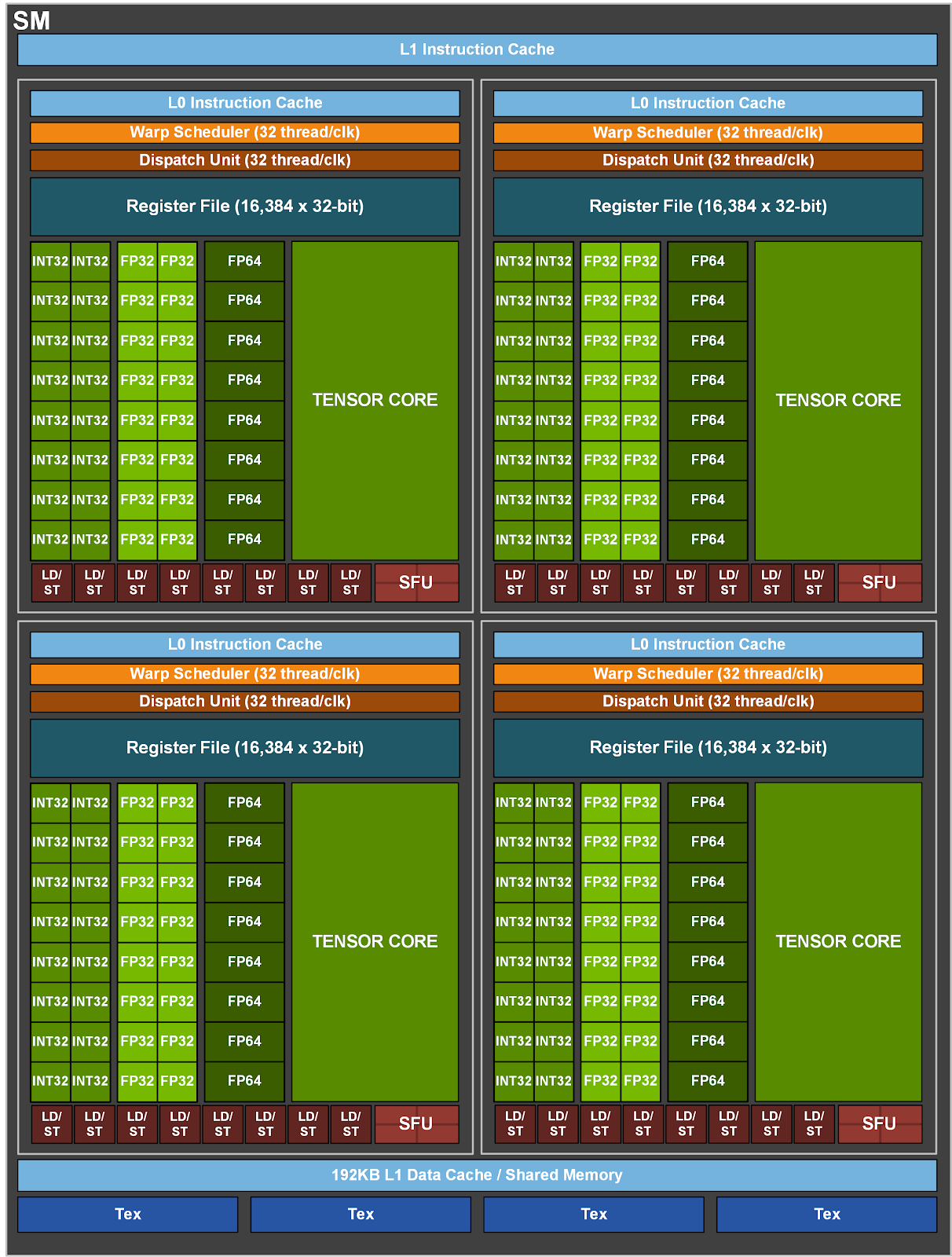
At the lower level you have a Streaming Processor (SP). He is part of a group of 16 SP which computes the same sequence of instructions at the same time.

(To be more precise, you have 16 FP32 cores, 8 FP64 cores, 16 INT32 cores, 1 Tensor Core, and 1 texture unit per group. More on tensor cores later)

The first constraint is the following: the 16 SP in the group cannot diverge from a single sequence instruction. This is called SIMD: Same Instruction, Multiple Data. That’s not exactly true, the instructions can contain “if“ statement, but if different branches are taken, some compute will be lost because every processor will have to execute both branches, and throw the results that are not useful for its own work.

4 groups of 16 SPs form a Streaming Multiprocessor (SM). Each group executes the same kernel (=function), but not in a strictly synchronized way. Still, you’ll have at least 64 cores working on the same task, or you’ll lose some computing capacity.

Then, you group 2 SMs to form a “Texture Processing Cluster” (TPC), and you group 8 TPCs to form a GPC (GPU Processing Cluster). 8GPCs and you have an A100 GPU. Pfew!

To sum it up, there are 128 SMs in an A100, so 8192 FP32 cores, but as you can see, we are far from getting a flat set of “8192” cores! (those are maximum numbers, first processors won’t have the full set of cores).

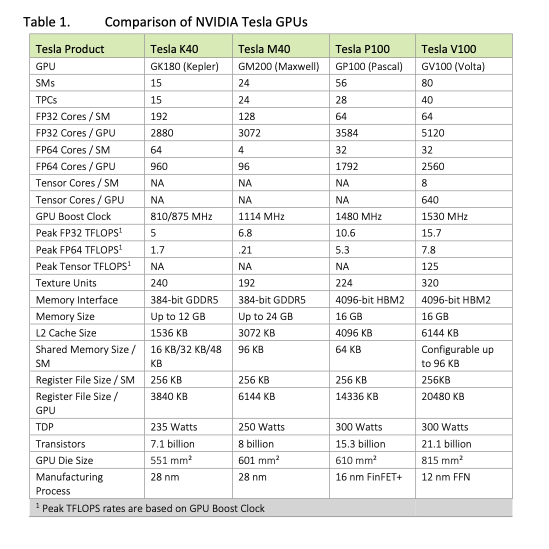
If you compare the A100 structure with the Volta V100, these structural numbers are almost the same, except for the PCs, and so for the grand total of course. The innards of the cores of course have changed too, but it looks like that the communication structure of the V100 was considered quite good for the kind of job it’s usually given. The Tensor Cores seems to be the area where the most innovation is taking place (more on this later).

You can see in the comparison below that all those numbers varied significantly with time, in search of the best performance :

Why so many levels? Performance

The main reason is of course to improve real-life performance. And in real life, you don’t have a single task to be done.

First, there may be several processes using your GPU at the same time on your machine. Not sure if it’s a good idea to get some good performance, but it’s of course something very usual.

In the new Ampere GPU, you can even partition your GPU to server multiple Virtual Machines with strong guarantees on your data security: the new feature is called “Multi-Instance GPU”.

In a single process, if your network contains several layers, some linear, some non-linear, some embedding, each one will use one or several kernels to do its job.

You may think that they are executed one after the other. It’s true to some extent, but in order to keep your GPU busy, your CPU is sending a stream of tasks to be done, not a task after the other, and the GPU will do them without the CPU waiting for each one to complete.

The CPU will basically wait after a full batch has been processed, after the forward and backward pass, because he has to update the full model before starting a new batch.

There are several reasons to have this “stream of task” model:

• The first reason is that starting a task takes some time, so the GPU can prepare the next task before the previous is started: changing the active kernel on some part of the GPU takes some time, pipelining saves time.

• Second, in the task stream, some tasks are not dependent on each other, so both can be executed in parallel in the GPU, so more work to be done, so less chance some part of the GPU is idling. Some networks are very, very parallel to compute, like Transformers, and so their efficiency is very good:

• there are only a few different layers, so few kernel changes and a lot of work for each kernel
• there are only loose dependencies between computations (eg for each token), so the GPU has a lot of degrees of freedom when scheduling the different parts of the computation: if a kernel is waiting for some data, maybe another one can compute its result because it already has its own data available.

  Why so many levels? Economics

Another reason is that it’s hard to get zero-defect silicon at this level of detail.

Ampere GPUs contain 54 billion transistors. Any defective transistor, and you may have to throw the GPU to the bin. The fraction of chips that pass the test is called the yield. Those chips are huge, and silicon real estate costs a lot, so each failed chip is a big loss, just for a small defect on a single transistor somewhere in the silicon.

So instead of throwing the chip to the bin, you test some sub-parts of the chip, and you just disable the failing sub-parts. That means, for example, disabling a GPC (remember, there are 7 of them in a A100, instead of a theoretical 8). And you sell it in a lower-end card, with reduced specs. This process is called binning. If you are really good, and your chips are all perfect, you may even disable perfectly working parts of your chip, to segment your offer (and back in time, some users were able to re-enable those disabled parts of silicon to get the bang without the buck…)

Developing for GPUs

So what are the consequences of the GPU architecture choices on development?

Kernels

First, you have to write some kernels, using the primitives you get. It’s a quite specific exercise, as you have to manually manage caches, registers, the synchronization of the different cores, etc. For simple stuff like matrix products, or activation layers, it’s quite straightforward, as they are completely parallel by nature.

But for some algorithms, like sorting, it can be a lot trickier to have something efficient, because you will have some issues using all the cores all the time.

Grids and performance

That’s because the kernel is only a small part of the problem, the other is the way you distribute the work among cores. And the performance gains are often made more on the distribution than on an optimal kernel.

The way you distribute the work is usually done by partitioning your job into a 2D or 3D grid, then mapping each point of the grid to a thread, and finally mapping those threads to physical cores. Those dimensions will correspond for example to the dimensions of the output of a layer, plus the batch dimension.

As you have seen, in a GPU you get thousands of cores to work with, but with a really complex multi-layered structure. And this structure change according to the generation and model of the GPU. So it’s hard to find the right way to choose those mappings. You often have to make some benchmarks to find the right way to do a computation with given dimensions on a specific GPU, and that information will be used in the future to choose the best strategy at runtime.

Memory

But the main and the most difficult hurdle a developer face while developing for GPU’s architecture is managing memory. And specifically memory transfers. The available memory bandwidth is huge, but the computing power is even larger. And just as you did not get a flat space of computing cores, you don’t get completely random access to the memory for free.

If you want to access a float number stored in the main memory from a GPU core, you will wait literally for ages compared to the time it takes to compute a sum or a multiply. So you need to be able to start hundreds of computations at once, and when the data is finally available, you resume your kernel, you execute a few local operations, until you need some more data from the main memory.

Some special ops like “prefetch” exist, to declare that you will need some data in a few instructions, and the role of the compiler is to reorder the instructions so you keep the memory controllers busy while keeping the core busy too. And at runtime, a large part of the GPU silicon is devoted to handling all those threads that are “in flight” and their current memory requests.

But there are some low-level constraints that may cost you a lot. Just like the base computation unit is 16 cores doing the same job, you really get peak memory performance if you load memory by quite large contiguous blocks, for example, 16 floats = 64 bytes, by a group of threads (called warp in CUDA lingo). This is called coalesced access. This is another reason, and often the main one, why choosing the right grid to dispatch your task on is important.

So now, let’s unroll back to our initial issue if you still remember (I would forgive you, I can barely): why sparse matrices ops are slow?

If you look at the memory access pattern you need to make a sparse matrix/ matrix multiplication, you’ll see that by definition it’s hard to have those blocks of 16 floats when reading the matrix weights. And reading 16 contiguous floats is just a minimum, you’ll need to read more data at once to reach full performance.

That explains why a naive implementation can be at least an order of magnitude slower than the dense version.

Unless you make some compromise and use a block sparse matrix: each block, if large enough, will produce large contiguous accesses. 8x8 blocks is a minimum in OpenAI implementation, but you will get even better performance with 32x32 blocks.

But of course, you have to make sure that your model is working in a similar fashion with block sparse compared to pure sparse matrices. It can be the case if your matrices are large enough so block size is small in comparison, but you have to check.

The other way is to convince an executive at Nvidia to add some hardware sparse support into their next-gen GPU, and now it’s done. More on this below!

Inter-GPU memory transfer

Memory bottlenecks exist within the GPU, but if you work with multiple GPUs sharing a single model, the available bandwidth is way lower than between memory and cores.

The DataParallel node of PyTorch is convenient, but it is no magic: after each batch, the GPUs must send their gradients to a single GPU, and then this latter must broadcast the updated model to each GPU. If your model is big enough, this transfer can take very significant time, and the performance will suffer. Another point is that the transfers are synchronous, no GPU can work if the new model has not been received.

Another way to use multiple GPUs is to split a single model between the different GPUs, and then transfer only the “frontier” layers from a GPU to the next. Same thing for backpropagation. This may not be ideal either as the first layer will have to wait for the last to complete before the backpropagation can occur. The performance will depend heavily on the morphology of the network.

Ampere Highlights

Let’s finish where we started, with the latest Nvidia announcement.

Tensor Cores

With Volta, Nvidia introduced new “Tensor Core units”, and it looks like they are here to stay. Turing and now Ampere iterated on these new units.

You can see them as ultra-specialized units, with some significant dedicated silicon.

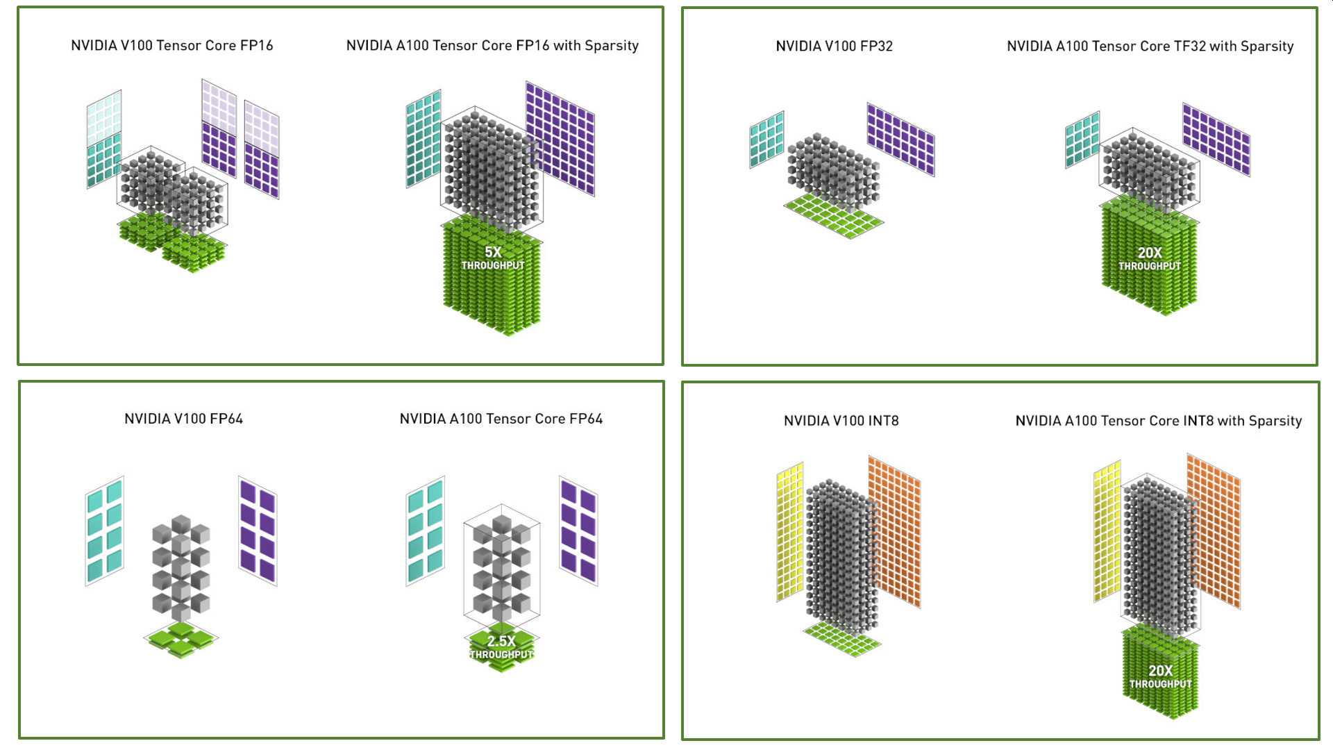
And this means a lot in terms of speed, especially quantized networks inference :

For training, it was a bit more difficult on Volta, as working with FP16 was possible but a bit tricky (the 8x gain in speed was indeed tempting).

But now with Ampere, Nvidia announces support for FP32 and even FP64 for Tensor Cores. And it looks like FP32 is now 20 times faster than on Volta with sparsity, and 10 times without sparsity. And this is for training and inference because it’s just big tensor ops, nothing special here.

It looks like we’ll be getting some nice toys to play with.

Sparsity

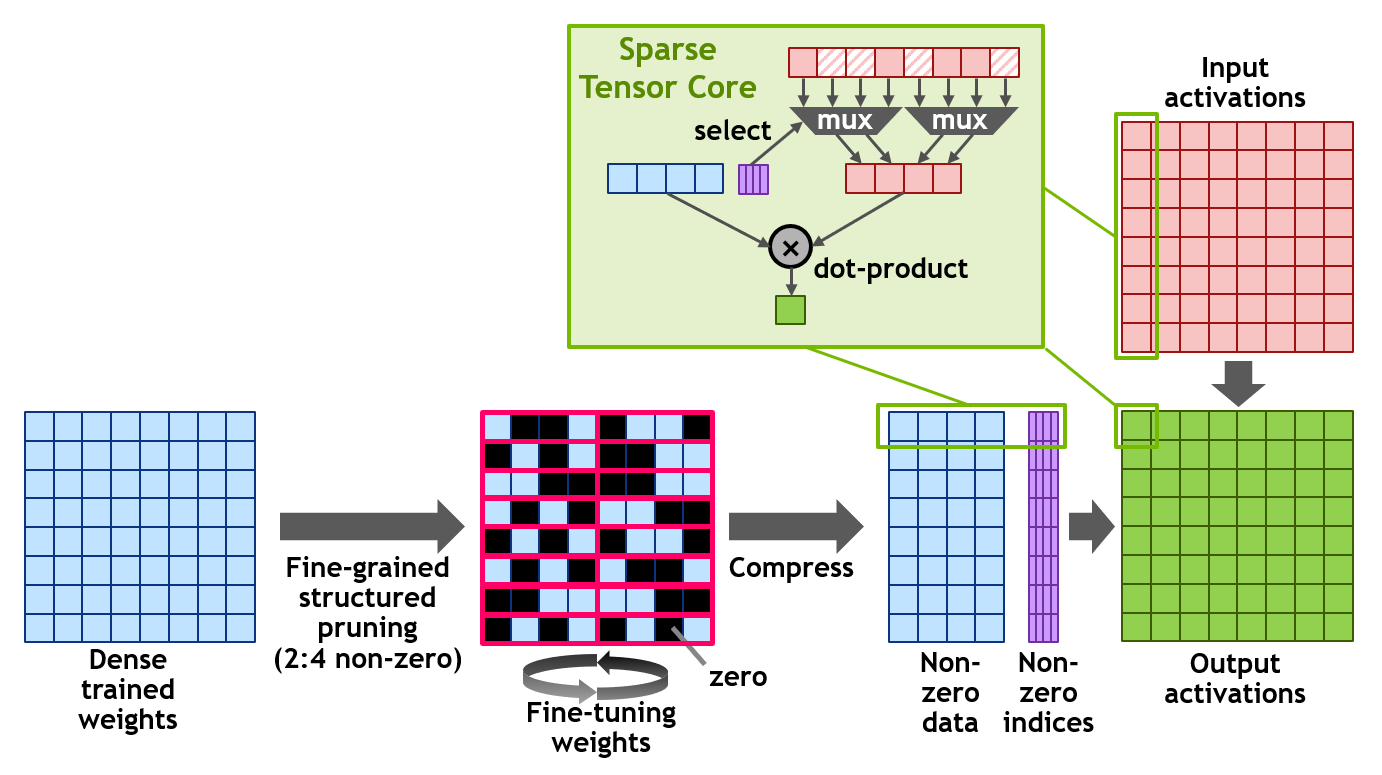
From the Nvidia Blog :

NVIDIA has developed a simple and universal recipe for sparsifying deep neural networks for inference using this 2:4 structured sparsity pattern.

If you have read the first part of this series, you should feel at home.

The idea is simple: maybe using a fully dense matrix is not useful. And what Nvidia is claiming is that it’s true, keeping only half the weights has a minimal impact on precision.

And so they propose a method to reduce the number of weights. But what is more interesting, is that the A100 GPU has new instructions to process efficiently these sparse matrices, at twice the speed of dense ones (no magic here, only half the multiply occurs of course).

So anyone can try its own method to sparsify the matrices and use the new instructions to speed things up. The only constraint is that the sparse pattern is fixed, as every 4 cells must have 2 sparse ones at most.

You can compare this to the way textures are compressed to save memory but for floating computation and not just graphics.

I see it mostly for inference at first, but I am sure some clever people will come with imaginative ways to use those new capabilities for training too, as it’s just some new compute ops.

What about “sparse block sparse matrices”, by combining soon to be released OpenAI “block sparse matrices” with this? We’ll see.

Conclusion

I hope you enjoyed this second part of our trip to sparse land, even if it may have been a bit harder to digest.

I hope too this will help you to better understand the level of mastery developers in the PyTorch or Keras team show: they manage to hide all this complexity and make it easy for mere mortals to use these supercomputer-on-a-chip to their full power, in just a few lines of python.

Next time we will get back to more usual depths: we’ll see some techniques we can use to train sparse networks, and how performance is impacted.

By the way, congrats to Victor Sanh, Thomas Wolf, and Alexander M. Rush for their latest paper “Movement Pruning: Adaptive Sparsity by Fine-Tuning”!